Contents

• Low Code Time Series Analysis
  • Using Darts to streamline your Python time series analysis development
• Introduction
• Demonstration
  • Data Preprocessing
  • Anomaly Detection
  • Baseline Model
  • Statistical Models selection
  • Backtesting
  • Covariates Analysis
• Bibliography

Photo by Afif Ramdhasuma on Unsplash

Low Code Time Series Analysis

Using Darts to streamline your Python time series analysis development

Introduction

Time Series Forecasting is a unique field in Machine Learning. When working with time series in fact there is an inherent time dependency between the different points in the series and therefore the different observations are highly dependent on each other. If you are interested in learning more about the basics of time series analysis, additional details can be found in this my previous article.

In the case of classical classification and regression problems scikit-learn is able to provide most of the utils we might need to get started with a good baseline (e.g. data pre-processing, low code models. evaluation metrics, etc…), although with time series the story is quite different. Many specialized libraries have become available throughout the years to cover some of the key steps in a Time Series Analysis workflow (e.g. statsmodels, Prophet, custom backtesting, etc…) but until Darts was not possible to cover everything within a single solution.

Demonstration

As part of this article, we are going to walk through a practical demonstration of how to use Darts to analyze the Delhi Daily Climate time series dataset from Kaggle [1]. All the code used throughout this article (and more!) is available on my GitHub and Kaggle accounts.

First of all, we need to make sure to have Darts installed in our environment.

pip install darts

Data Preprocessing

At this point, we are ready to import the necessary libraries and datasets (Figure 1). In order to facilitate our analysis, the date column is first converted from string to datetime and then set as the index of the dataframe.

import numpy as np
import pandas as pd
from matplotlib import pyplot as plt
import darts
from darts.ad import QuantileDetector

df = pd.read_csv('DailyDelhiClimateTrain.csv')
df["date"] = pd.to_datetime(df["date"])
df = df.set_index('date')
df.head(5)

Figure 1: Delhi Daily Climate time series dataset (Image by Author).

Once cleaned the dataset, we can now divide it into training and test subsets and visualize the time series (Figure 2). For our analysis, we are just going to focus on the mean temperature for the moment.

ts = darts.TimeSeries.from_series(df.meantemp)
train, val = ts.split_before(0.75)
train.plot(label="Training Data")
val.plot(label="Validation Data")

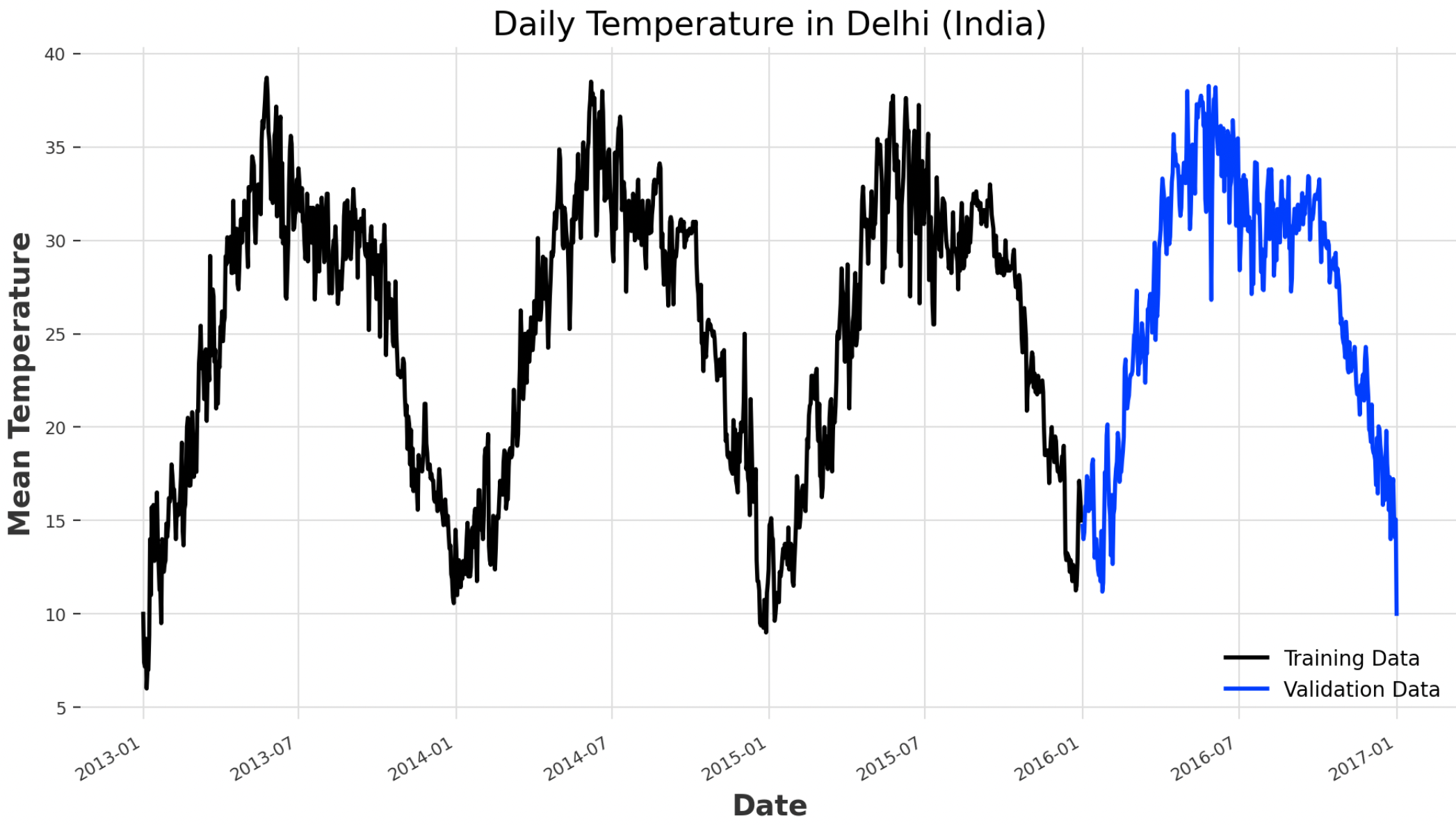
Figure 2: Daily Temperature in Delhi Time Series (Image by Author).

Anomaly Detection

Due to their nature, time series are usually processed as part of real-time or streaming services, this can although make them more susceptible to wrong measurements and the generation of outliers. In order to monitor our time series for possible abnormal values, different anomaly detection techniques can be used. Two possible approaches are using quantiles or thresholds. With quantiles, we decide to flag the top and bottom percent of our values in the series as outliers, while with thresholds we specify fixed reference levels above or below which each value is flagged as anomalies.

In the example below, considering anything below 3% and above 97% as outliers leads to an overall percentage of values outside quantiles of 5.8% (Figure 3).

anomaly_detector = QuantileDetector(low_quantile=0.03, high_quantile=0.97)
anomalies = anomaly_detector.fit_detect(ts)

l = anomalies.pd_series().values
print("Percentage of values outside quantiles:", 
        round(sum(l)/len(l)*100, 3), "%")

idx = pd.date_range(min(ts.pd_series().index), max(ts.pd_series().index))
anomalies = ts.pd_series()[np.array(l,dtype=bool)].reindex(idx,
                                                            fill_value=np.nan)
normal = ts.pd_series()[~np.array(l,dtype=bool)].reindex(idx, 
                                                            fill_value=np.nan)

normal.plot(color="black", label="Normal")
anomalies.plot(color="red", label="Anomalies")

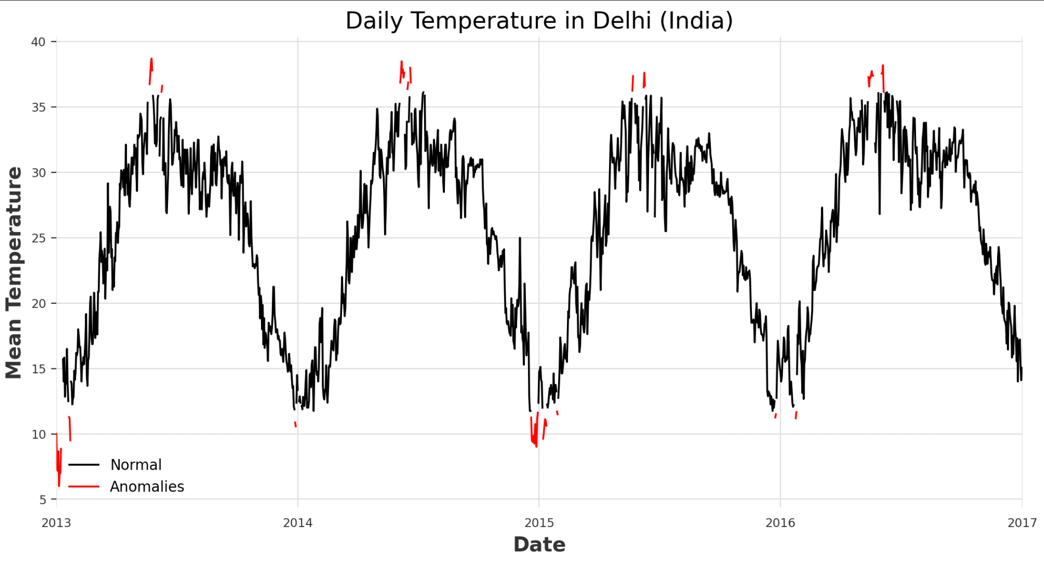
Figure 3: Quantile Anomaly Detection (Image by Author).

Baseline Model

At this point, we are ready to dive deeper into our time series and check if it’s present any form of seasonality. As expected and shown in the code snippet below, the series seems to statistically follow a similar seasonal pattern approximately every year.

for m in range(2, 370):
        seasonal, period = darts.utils.statistics.check_seasonality(train, 
                                                m=m, max_lag=400, alpha=0.05)
        if seasonal:
            print("Seasonality of order:", str(period))

Seasonality of order: 354
Seasonality of order: 356
Seasonality of order: 361

Given this information, we can train a first naive baseline model which just takes into account the seasonal pattern in the series and no other information (Figure 4). Using this approach, results in 11.35% MAPE (Mean Absolute Percentage Error). Two of the main advantages of using MAPE as our evaluation metrics are:

• Using the absolute value, positive and negative errors are not canceled out.

• The errors are not dependent on the scaling of the dependent variable.

k = 361
naive_model = darts.models.NaiveSeasonal(K=k)
naive_model.fit(train)
naive_forecast = naive_model.predict(len(val))

print("MAPE: ", darts.metrics.mape(ts, naive_forecast))
ts.plot(label="Actual")
naive_forecast.plot(label="Naive Forecast (K=" + str(k) + ")")

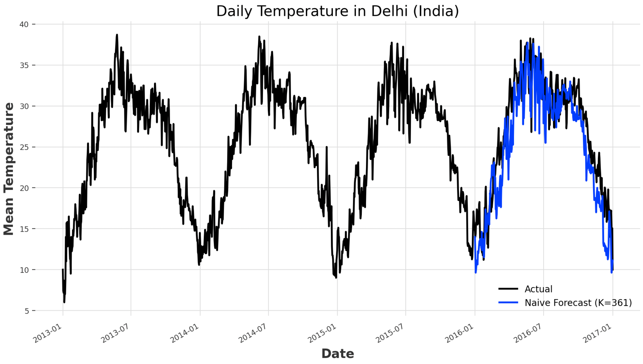
Figure 4: Baseline Model Forecasting (Image by Author).

Statistical Models selection

Provided now with a good baseline model, we are ready to experiment with some more advanced techniques (e.g. Exponential Smoothing, ARIMA, AutoARIMA, Prophet). If needed, many additional models such as: CatBoost, Kalman Filters, Random Forests, Recurrent Neural Networks, and Temporal Convolutional Networks are available as part of Darts.

def model_check(model):
    model.fit(train)
    forecast = model.predict(len(val))
    print(str(model) + ", MAPE: ", darts.metrics.mape(ts, forecast))
    return model

exp_smoothing = model_check(darts.models.ExponentialSmoothing())
arima = model_check(darts.models.ARIMA())
auto_arima = model_check(darts.models.AutoARIMA())
prophet = model_check(darts.models.Prophet())

ExponentialSmoothing(), MAPE:  37.758
ARIMA(12, 1, 0), MAPE:  41.819
Auto-ARIMA, MAPE:  32.594
Prophet, MAPE:  9.794

Given the results above, Prophet seems to be the most promising of the models considered so far as part of the analysis. In any case, with some additional work, the results could even be improved using Hyper-parameter optimization, especially by taking advantage of business domain knowledge with traditional statistical models such as ARIMA and Exponential Smoothing. Additional details about how ARIMA works and its different hyperparameters can be found here.

Backtesting

In order to further validate the goodness of our model, we can now test it by playing it out using the available historical data (Figure 5). In this case, a MAPE of 7.8% is registered.

historical_fcast = prophet.historical_forecasts(ts,
                            start=0.6, forecast_horizon=30, verbose=True)

print("MAPE: ", darts.metrics.mape(ts, historical_fcast))
ts.plot(label="Actual")
historical_fcast.plot(label="Backtest 30 days ahead forecast")

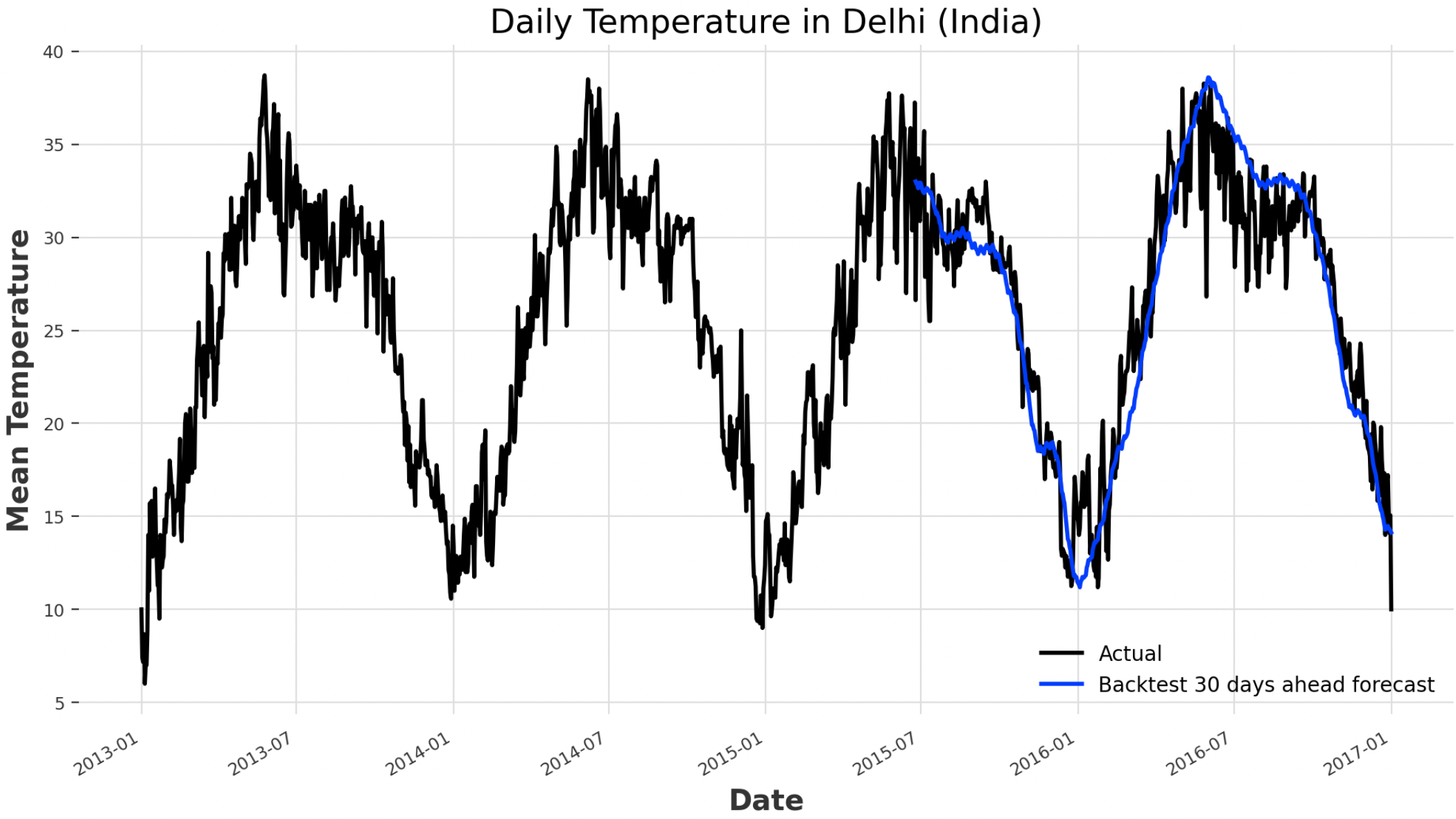
Figure 5: Prophet Backtesting (Image by Author).

Covariates Analysis

To conclude our analysis, we can now check if using the information stored in the other columns of the dataset such as the humidity and wind speed could help us to create a more performant model. There are 2 main types of covariates: past and future. With past covariates, just the past values are available at prediction time, instead with future covariates also future values are available at prediction time.

In this example, the N-BEATS (Neural Basis Expansion Analysis Time Series) model is used with the humidity and wind speed columns used as past covariates (Figure 6).

humidity = darts.TimeSeries.from_series(df.humidity)
wind_speed = darts.TimeSeries.from_series(df.wind_speed)

cov_model = darts.models.NBEATSModel(input_chunk_length=361, 
                                        output_chunk_length=len(val))
cov_model.fit(train, past_covariates=humidity.stack(wind_speed))
cov_forecast = cov_model.predict(len(val), 
                                past_covariates=humidity.stack(wind_speed))

print("MAPE: ", darts.metrics.mape(ts, cov_forecast))
ts.plot(label="Actual")
cov_forecast.plot(label="Covariate Forecast")

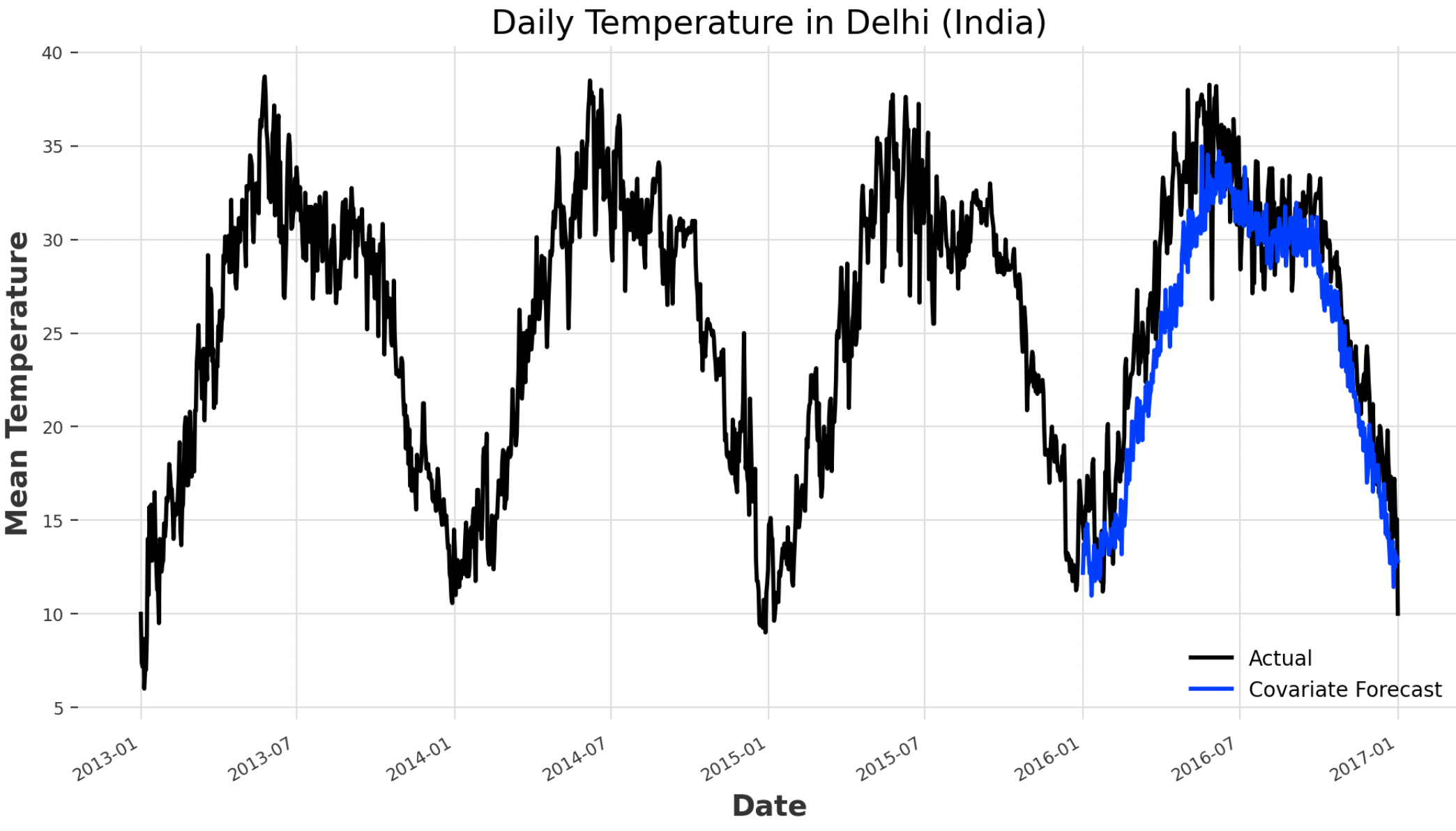
Figure 6: Covariates Analysis Forecasting (Image by Author).

As a result of the training process, a MAPE score of 10.9% is registered, therefore underperforming our original Prophet model in this occasion.

Bibliography

[1] “Daily Climate time series data” (SUMANTHVRAO, License CC0: Public Domain). Accessed at: https://www.kaggle.com/datasets/sumanthvrao/daily-climate-time-series-data?select=DailyDelhiClimateTrain.csv

Contacts

If you want to keep updated with my latest articles and projects follow me on Medium and subscribe to my mailing list. These are some of my contacts details:

• LinkedIn
• Patreon
• Medium Profile
• GitHub
• Kaggle

Share with friends

Linkedin Twitter Facebook Reddit Email