Contents
Interactive Data Visualization
Creating interactive plots and widgets for Data Visualization using Python libraries such as: Plotly, Bokeh, nbinteract, etc…
Data Visualization
Data Visualization is a really important step to perform when analyzing a dataset. If performed accurately it can:
- Help us to gain a deep understanding of the dynamics underlying our dataset.
- Speed up the machine learning side of the analysis.
- Make easier for others to understand our dataset investigation.
In this article, I will introduce you to some of the most used Python Visualization libraries using practical examples and fancy visualization techniques/widgets. All the code I used for this article is available in this GitHub repository.
Matplotlib
Matplotlib is probably Python most known Data Visualization library. In this example, I will walk you through how to create an animated GIF of a PCA variance plot.
First of all, we have to load the Iris Dataset using Seaborn and perform PCA. Successively, we plot 20 graphs of the PCA variance plot while varying the angle of observation from the axis. In order to create the 3D PCA result plot, I followed The Python Graph Gallery as a reference.
Finally, we can generate a GIF from the 20 graphs we produced using the following function.
The result obtained should be the same as the one in Figure 1. This same mechanism can be applied in many other applications such as: animated distributions, contours, and classification machine learning models.
Figure 1: PCA variance plot
Another way to make animated graphs in Matplotlib can be to use the Matplotlib Animation API. This API can allow as to make some simple animations and live graphs. Some examples can be found here.
Celluloid
Celluloid library can be used in order to make animations easier in Matplotlib. This is done by creating a Camera aimed to take snapshots of a graph every time one of its parameters changes. All these pictures are then momentarily stored and combined together to generate an animation.
In the following example, a snapshot will be generated for every loop iteration and the animation will be created using the animate() function.
It is then also possible to store the generated animation as a GIF using ImageMagick. The resulting animation is shown in Figure 2.
Figure 2: Celluloid Example
Plotly
Plotly is an open-source Python library built on plotly.js. Plotly is available in two different modes: online and offline. Using this library we can make unlimited offline mode charts and at maximum 25 charts using the online mode. When installing Plotly, it is although necessary to register to their website and get an API key to get started (instead of just using a pip install like for any other libraries considered in this article).
In this post, I will now walk you through an example using the offline mode to plot Tesla stock market High and Low prices over a wide span of period. The data I used for this example can be found here.
First of all, we need to import the required Plotly libraries.
Successively, I imported the dataset and preprocessed it in order to then realize the final plot. In this case, I made sure the columns I wanted to use for the plot were of the right data-type and the dates were in the format (YYYY-MM-DD). To do so, I converted the High and Low prices columns to double datatypes and the Date column to a string format. Successively I converted the Date column from a DD/MM/YYYY format to YYYY/MM/DD and finally to YYYY-MM-DD.
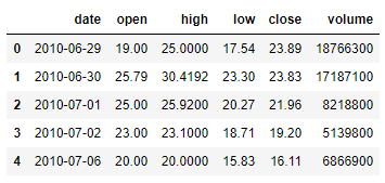
Figure 3: Tesla Dataset
Ultimately, I used the Plotly library to produce a Time Series chart of Tesla’s stock market High and Low prices. Thanks to Plotly, this graph will be interactive. Placing the cursor on any point of the time series we can get the High and Low prices and using either the buttons or the slider we can decide on which timeframe we want to focus on.
In Figure 4 is shown the final result. Plotly documentation offers a wide range of examples on how to make the best out of this library, some of these can be found here.
Figure 4: Plotly Example
Bokeh
Bokeh library is available for both Python and JavaScript. Most of its graphs, interaction and widgets can be implemented just using Python but in some cases might be necessary to use also Javascript.
When using Bokeh, graphs are built by stacking one layer on top of another. We first start by creating a figure and then we add elements on it (Glyphs). Depending on the plot we are trying to make, Glyphs can be of any form and shape (eg. lines, bars, circles).
When creating plots using Boker, some tools get automatically generated along with the plot. These are: a reference link to the Bokeh documentation, a pan, a box zoom, a wheel zoom, a save option and a reset graph button (same as Plotly).
As a practical example, I will now walk through how to make an interactive time series plot using the same dataset used in the Plotly example.
For this demonstration, will be plotted four different time series (High/Low/Open and Close Price) and will be created four checkboxes. In this way, the user will have the option to check/uncheck the boxes to make any of the four-time series disappear from the graph.
In this example, in order to implement the checkboxes functionalities, Javascript was used instead of Python.
The resulting plot is shown in Figure 5.
Figure 5: Bokeh Demonstration
As shown in the code above, the plot has additionally been saved as an HTML file. This same option can be applied to Plotly graphs as well. If you are interested to test yourself the plots realized with Plotly and Bokeh, they are available here.
Both Plotly and Bokeh can be additionally used as dashboard frameworks for Python, creating quite astonishing results [1, 2].
Seaborn
Seaborn is a Python library built upon Matplotlib used to make statistical graphs. According to Seaborn’s official website:
If Matplotlib “tries to make easy things easy and hard things possible”, Seaborn tries to make a well-defined set of hard things easy too.
I will now walk you through a simple example using Seaborn. If you are looking to find out more about this library, Seaborn example gallery is a great place where to start.
In the following example, I first loaded the Iris Dataset using Seaborn and then created a pair-plot.
A pair-plot is a function able to provide a graphical summary of the variable pairs in a dataset. This is done by using scatterplots and a univariate distribution representation of the matrix diagonal. In Figure 6 are shown the results of this analysis.
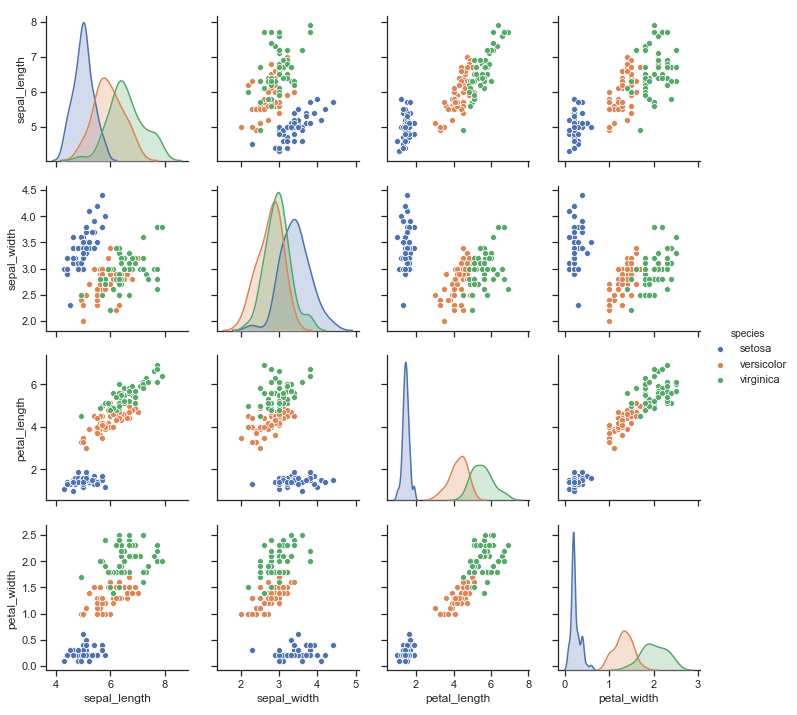
Figure 6: Seaborn Pair-plot
nbinteract
nbinteract enables us to create interactive widgets in Jupiter Notebook. These widgets can also be exported in HTML if wanted. An example of an online implementation of nbinteract can be found here.
As a simple implementation here will be created a drop-down menu. Changing the selection of the number of cars or the name of the owner will update in real-time the string (Figure 7).
Figure 7: NBInteract Example
Moving from Python 3.9 onwards, Jupyter Widgets might provide better support for out of the box widget consumption in Notebook based environments.
Additional Libraries
In addition to the libraries already mentioned, also Pygal and Altair are other two Python libraries commonly used. They both provide similar kind of plots to the ones shown before, but can additionally be used to create other forms of plots such as: Pyramids, Treemaps, Maps and Gantt Charts.
Bibliography
[1] Bokeh — Gallery, Server App Examples. Accessed at: https://bokeh.pydata.org/en/latest/docs/gallery.html
[2] Plotly — Dash App Gallery. Accessed at: https://dash-gallery.plotly.host/Portal/
Contacts
If you want to keep updated with my latest articles and projects follow me on Medium and subscribe to my mailing list. These are some of my contacts details:
