Contents
GPU Accelerated Data Analytics & Machine Learning
The future is here! Speed up your Machine Learning workflow using Python RAPIDS libraries support.
Introduction
GPU acceleration is nowadays becoming more and more important. The main two drivers for this shift are:
- The world’s amount of data is doubling every year [1].
- Moore’s law is now coming to an end because of limitations imposed by the quantum realm [2].
As a demonstration for this shift, an increasing number of online data science platforms is now adding GPU enabled solutions. Some examples are: Kaggle, Google Colaboratory, Microsoft Azure and Amazon Web Services (AWS).
In this article, I will first introduce you to the NVIDIA open-source Python RAPIDS libraries and I will then offer you a practical demonstration of how RAPIDS can speed up Data Analysis up to 50 times.
All the code used for this article is available on my GitHub and Google Colaboratory for you to play with.
RAPIDS
Many solutions have been proposed in the last few years in order to work with large amounts of data. Some examples are MapReduce, Hadoop and Spark.
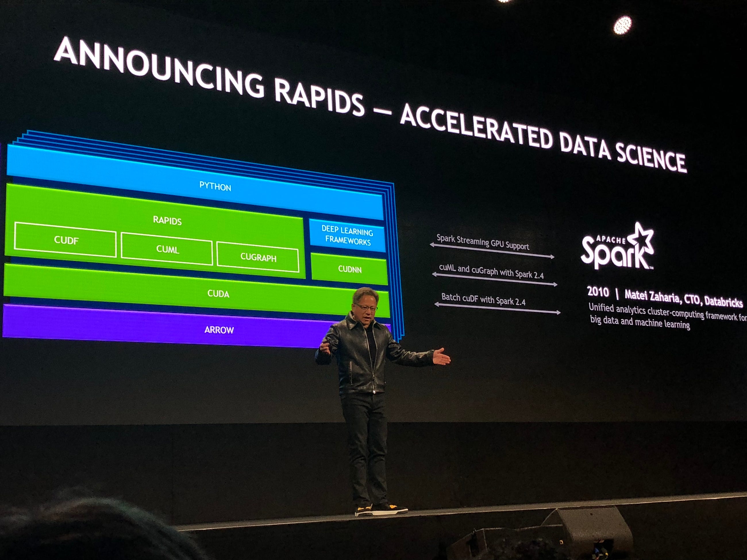
RAPIDS is now designed to be the next evolutionary step in data processing. Thanks to its Apache Arrow in-memory format, RAPIDS can lead to up to around 50x speed improvement compared to Spark in-memory processing (Figure 1). Additionally, it is also able to scale from one to multi-GPUs [3].
All RAPIDS libraries are based on Python and are designed to have Pandas and Sklearn like interfaces to facilitate adoption.
 Figure 1: Data Processing Evolution [3]
All RAPIDS packages are now free to be used on Anaconda, Docker and cloud-based solutions such as Google Colaboratory.
RAPIDS structure is based on different libraries in order to accelerate data science from end to end (Figure 2). Its main components are:
- cuDF = used to perform data processing tasks (Pandas like).
- cuML = used to create Machine Learning models (Sklearn like).
- cuGraph = used to perform graphing tasks (Graph Theory).
RAPIDS has additionally integration with: PyTorch & Chainer for Deep Learning, Kepler GL for visualization, and Dask for distributed computation [4].
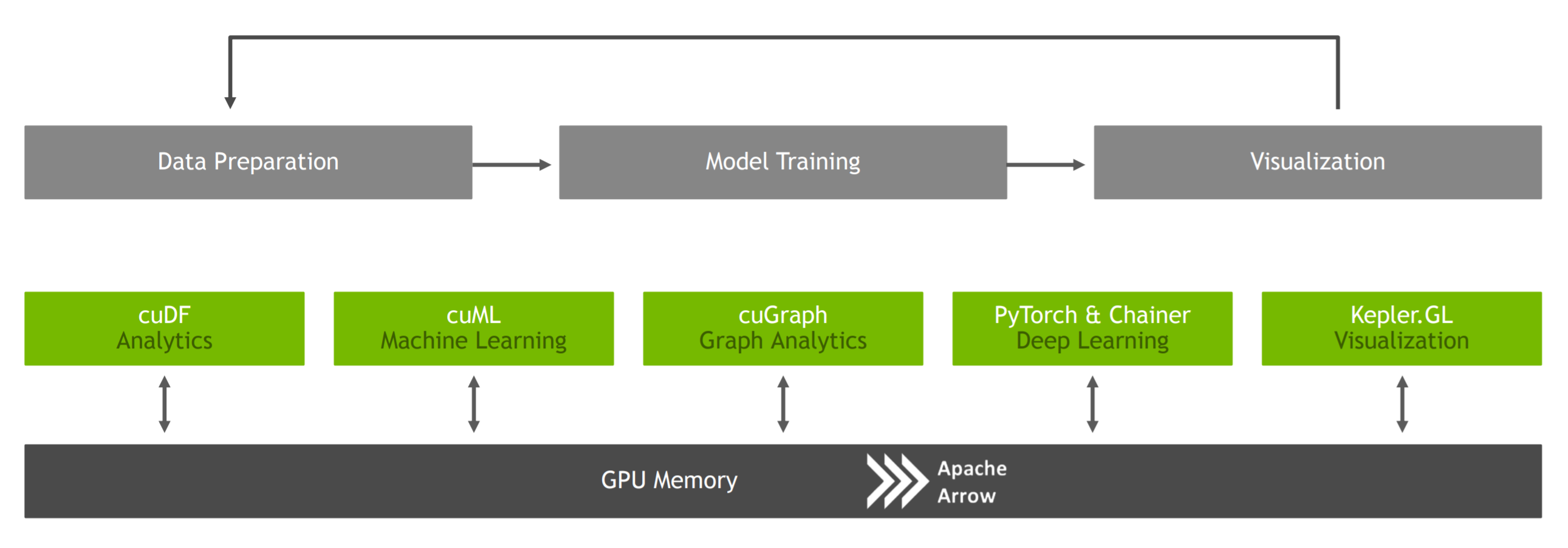 Figure 2: RAPIDS architecture [3]
Demonstration
I will now demonstrate to you how using RAPIDS can lead to a faster Data Analysis compared to using Pandas and Sklearn. All the code I will be using is available on Google Colaboratory, so feel free to test it out yourself!
In order to use RAPIDS, we need first of all to enable our Google Colaboratory notebook to be used in GPU mode with a Tesla T4 GPU and then install the required dependencies (guidance is available on my Google Colabortory notebook).
Preprocessing
Once is everything set up, we can then import all the necessary libraries.
In this example, I will show you how RAPIDS can speed up your Machine Learning workflow compared to just using Sklearn. In this case, I decided to use Pandas for preprocessing both the RAPIDS and Sklearn analysis. On my Google Colaboratory notebook is available also another example in which I use instead cuDF for preprocessing. Using cuDF instead of Pandas, can lead to faster preprocessing especially if working with a large amount of data.
For this example, I decided to fabricate a simple dataset using Gaussian Distributions consisting of three features and two labels (0/1).
The values of the means and standard deviations of the distributions have been chosen so that to make this classification problem fairly easy (linearly separable data).
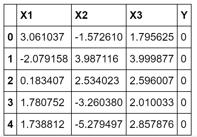
Figure 3: Sample Dataset
Once created the dataset, I divided it features and labels and then defined a function to preprocess it.
Now that we got our Training/Test sets we are finally ready to get started with our Machine Learning. In this example, I will be using XGBoost (Extreme Gradient Boosting) as classifier.
RAPIDS
In order to use XGBoost with RAPIDS we need first to convert our Training/Tests inputs in matrix form.
Successively, we can start training our model.
The output of the above cell is shown below. Using the XGBoost library provided by RAPIDS took just under two minutes to train our model.
CPU times: user 1min 54s, sys: 307 ms, total: 1min 54s
Wall time: 1min 54s
Additionally RAPIDS XGBoost library provides also a really handy function to rank and plot the importance of each feature in our dataset (Figure 4).
This can be really useful in order to reduce the dimensionality of our data. By selecting just the most important features and training our model on it, we would, in fact, reduce the risk to overfit our data and we would also speed up training times. If you want to find out more about feature selection you can read this my article about it.
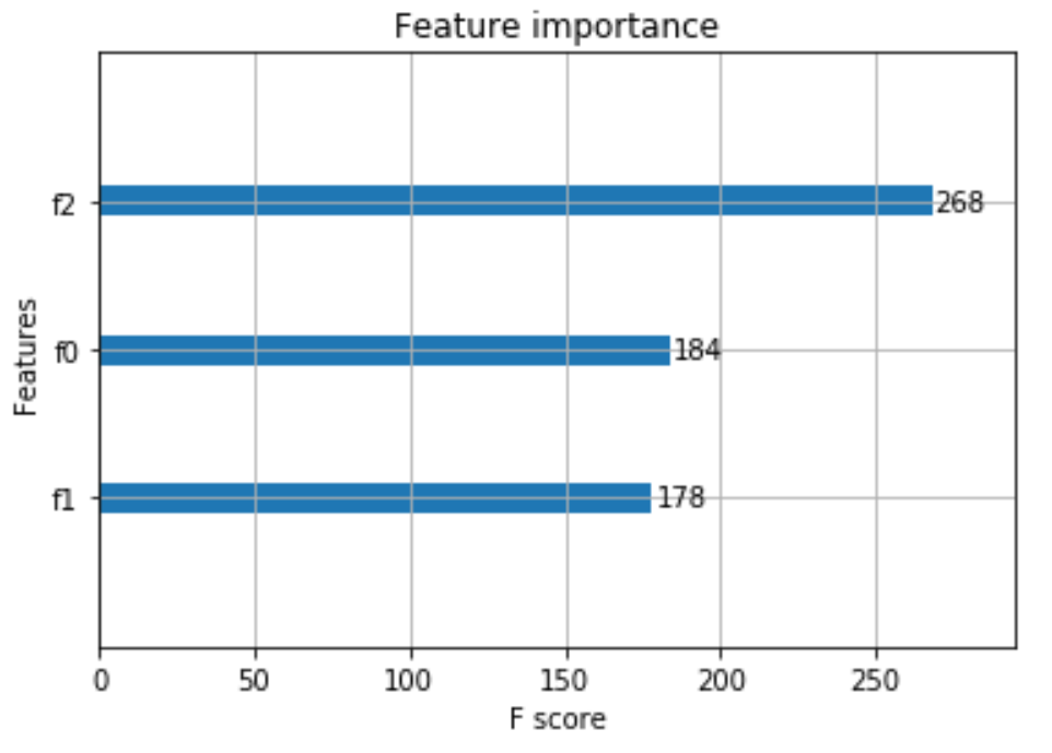 Figure 4: XGBoost Feature Importance
Finally, we can now calculate the accuracy of our classifier.
The overall accuracy of our model using RAPIDS was equal to 98%.
XGB accuracy using RAPIDS: 98.0 %
Sklearn
I will now repeat the same analysis using plain Sklearn.
In this occasion, it took just above 11 minutes to train our model. That means using Sklearn for this problem size was 5.8 times slower than using RAPIDS (662s/114s). By using cuDF instead of Pandas in the preprocessing stage we can reduce the execution time even more for the overall workflow of this example.
CPU times: user 11min 2s, sys: 594 ms, total: 11min 3s
Wall time: 11min 2s
Finally, calculated the overall accuracy of the model using Sklearn.
Also, in this case, the overall accuracy was equal to 98%. That means that using RAPIDS can lead to faster results without compromising at all our model accuracy.
XGB accuracy using Sklearn: 98.0 %
Conclusion
As we can see from this example, using RAPIDS lead to a consistent decrease in execution time.
This can be greatly important when working with large amounts of data since RAPIDS would be able to reduce execution time from days to hours and from hours to minutes.
RAPIDS offers valuable documentation and examples to make the most out of its libraries. If you are interested in finding out more, some examples are available here and here.
I additionally created two other notebooks to explore RAPIDS cuGraph and Dask libraries. If you are interested in finding out more, these are available here and here.
Bibliography
[1] What is Big Data? — A Beginner’s Guide to the World of Big Data. Anushree Subramaniam, edureka! . Accessed at: https://www.edureka.co/blog/what-is-big-data/
[2] No More Transistors: The End of Moore’s Law. Interesting Engineering, John Loeffler. Accessed at: https://interestingengineering.com/no-more-transistors-the-end-of-moores-law
[3] RAPIDS: THE PLATFORM INSIDE AND OUT, Josh Patterson 10–23–2018. Accessed at: http://on-demand.gputechconf.com/gtcdc/2018/pdf/dc8256-rapids-the-platform-inside-and-out.pdf
[4] GPU-Accelerated Data Science | NVIDIA GTC Keynote Demo. Jensen Huang. Accessed at: https://www.youtube.com/watch?v=LztHuPh3GyU
Contacts
If you want to keep updated with my latest articles and projects follow me on Medium and subscribe to my mailing list. These are some of my contacts details:
