Foundations of Data Structures and Algorithms

Foundations of Data Structures and Algorithms

“Computer Science is no more about computers than astronomy is about telescopes” –Edgar W.Dijkstra

What are data structures and algorithms?

Data Structure: a data organization, management, and storage format that enables efficient access and modification. More precisely, a data structure is a collection of data values, the relationship between them and the functions or operations which can be applied to the data (e.g. stack of books on top of each other).
Algorithm: a sequence of instructions, constructed to solve a class of problems or perform a computation. Algorithms are unambiguous specifications for performing calculations and data processing (e.g. the process of taking a series of books from a stack of books until we find the book we are looking for).

In short, a data structure is a way to organize information while an algorithm is a way to process information to reach an end goal.

Object Oriented Programming

Object: Instance of a class.
Class: Template for constructing objects (an abstraction of a real entity used to store and manipulate data however we think it is necessary). When we use a class to construct distinct objects, we call these objects instances.

Classes have two main components fields and methods. The fields describe the state of the object (e.g. length/width of a rectangle). The methods instead describe the behaviour of the object (e.g. a function created in order to modify the different parameters of a rectangle).

When trying to create complex programs, it might happen that different classes share similar characteristics. In this case, it might be useful to make use of inheritance (e.g. if we are creating a class for creating squares, and we already have a class for creating rectangles, then we can just inherit the information from the class to create rectangles and add some constrains to create a class to instantiate squares).

Primitive Operation: any operation that corresponds to a low-level instruction that runs in constant time (e.g. assigning a value to a variable, calling a method,..).

Analysis of Algorithms

Many computer science tasks are heavily based on algorithms. In order to decide if an algorithm is overall better than another for a specific task, it is then necessary to set up a consistent way to judge them. Using primitive operations takes time, and therefore when designing an algorithm we should aim to minimize as much as we can the number of times we use them (in order to make our algorithm run faster).

The key question we should ask ourselves in order to design good algorithms is: How does the number of primitive operations relate to the size of our input?

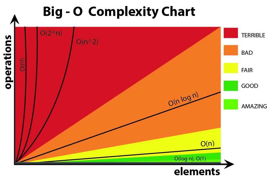
Big O notation: refers to the limiting behaviour of a function (worst case scenario). If we execute our algorithm multiple times and vary the input size, we can then plot the number of operations used to solve the problem against the number of provided input elements. The resulting curve will then represent which trend our algorithm follows as we increase the input size. Our objective in this case is to minimize the area under the curve (Figure 1). The Big O Notation can then be used to quantify the efficiency of the different algorithms. When we talk about the Big O Notation, we typically take into account the algorithm behaviour for very large input values (because of that we generally ignore constants).

Figure 1: Amitshahi.dev, Big ‘O’ Notation

Time complexities examples:

O(1): constant time (the runtime of the algorithm is not dependent on the size of the input). The plot will therefore be a flat spectrogram.
O(log(n)): we cut our input size in half repeatedly, which is modelled by log base two (e.g. binary search).
O(n): linear time (number of operations = input size).
O(nlog(n)): typically seen in sorting and divide and conquer style Algorithms (e.g. running something O(n), log(n) times or O(log(n)), n times).
O(n²): is slower than linear time and often occurs when working with 2 nested loops.

Classes of Running Times	Big O Notation
Constant	O(1)
Logarithmic	O(logN)
Linear	O(N)
Linearithmic	O(NlogN)
Polynomial	O(N²), O(N³), etc..
Exponential	O(2^N), O(3^N), etc..

This same type of reasoning can be applied not just to time complexity (how fast an algorithm runs), but as well to space complexity (how much memory it needs to run).

How to identify the running time of an algorithm?

Understand how the algorithm works (What is the purpose of the algorithm? What are the inputs/outputs?)
Identify a basic unit of the algorithm to count (e.g. print/iterations/assignment statements, recursive calls). The focus is on the worst case scenario.
Map the growth of count from step 2 to an appropriate Big O class (e.g. is the growth constant/exponential/linear/logarithmic?).

Dynamic Arrays

Dynamic Arrays are a fundamental data structure. The key feature of dynamic arrays is that they allow for efficient (fast) insertion/access/remove operations. This is a remarkable feature considering that computers under the hood works by using fixed length arrays (every time we need to resize our array we need to copy all the elements across and change the original memory size). In programming languages like Python and Java, an insertion/remove operation can run in O(N) (worst case, otherwise O(1) on average).

Recursion

In the world of problem solving, recursion is about taking a big problem and then breaking it down into smaller and smaller components until we reach a base case (e.g. factorial computation).

Therefore, a recursive function refers back to itself until reaching a base case (this generates a recursive trace, in which at each call information is stored about the computed result waited to be used once reached the base condition). One problem with using recursion is that each function call is stored on the stack trace (making too many calls to the recursive function could therefore potentially lead to memory issues in the long run).

5 steps to solve any recursive problem

What’s the simplest possible input? (The simplest case, often becomes our base case for the problem. The base case of a recursive function is the only input, for which we provide an explicit answer. All the other solutions to the problem will then build upon the base case.)
Play around creating different examples and try to visualize them.
Relate hard cases to simpler cases.
Generalize any underlying pattern we managed to undercover.
Write code by combining recursive patterns with the base case.

Graph Theory

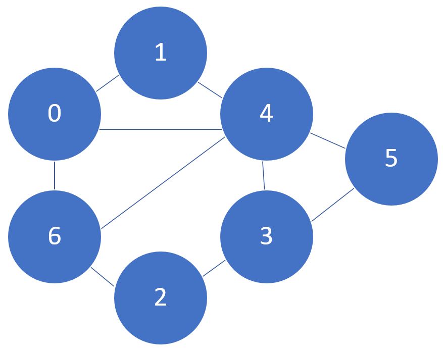
A graph is a network which can help us to define and visualize relationships between various components (Figure 2). Components are commonly referred in graph theory as vertices/nodes, while relationships are commonly referred as edges. Graph theory aims therefore to help in better understanding these type of networks and how they can be used in order to solve various problems (e.g. navigation, social networks, sudoku). Different nodes are considered to be neighbours if they are connected together by an edge. Each node can additionally be defined by its degree (number of neighbours).

Figure 2: Connected Graph

Another key characteristic of graphs are paths. A path can be defined as a sequence of vertices connected by edges and the path length is instead defined as the number of edges in a path. A special case of path is a cycle (a path that starts and ends at the same vertex). All cycles are paths but not all paths are necessarily cycles.

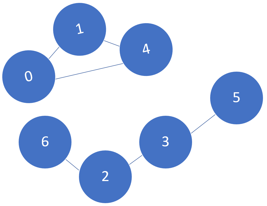
Graphs can be connected or not (Figure 3). A graph is connected if all vertices are connected (a path exists between all pair of vertices). Not connected graphs, can although still have connected components (a subset of vertices in a graph that is connected).

Figure 3: Not connected Graph

Types of Graphs

Undirected Graphs = edges are bidirectional.
Directed (Cyclic) Graphs = edges are unidirectional and there is a cycle.
Directed (Acyclic) Graphs = edges are unidirectional and there are no cycles.
Weighted Graphs = the edges of the graph are not treated equally and some edges might have an higher weight than others.
Trees = are a type of connected and acyclic graph. Removing an edge in a tree would disconnect the graph and adding an edge would create a cycle.

Graph representations

Graphs can be constructed in different ways when coding, some possible approaches are:

Map the different vertices into an adjacency matrix. If an edge exists between a row-column pair, this is represented as a 1, otherwise a 0 is stored in the matrix.
An edge set can be constructed in order to store the different connections (e.g. {(0, 1) (0, 2), (1, 2)}).
In an adjacency list, for each of the nodes in the graph is stored a list of all their neighbours. This is currently the most common way in order to represent a graph while coding.

Graph Algorithms

Depth First Search (DFS) and Breath First Search (BFS) are two types of Graph Traversal techniques (algorithms that visit every vertex of a graph). Graph Traversal techniques can either be Preorder (we mark a node as visited as soon as we encounter it) or Postorder (we mark a node as visited once we explored all his neighbours). Some example applications of DFS are: Cycle Detection, Finding Connected Components and Topological Sorting.

Dynamic Programming

Dynamic programming is one of the most powerful algorithmic programming techniques in computer science. The key idea behind dynamic programming is to try to solve a problem by first identifying and solving its related subproblems. Bringing together all the subproblems it would then be possible to solve the bigger problem. In order to try to solve dynamic programming problems, 5 key steps can be usually followed:

Visualize the problem through examples (e.g. using which data structure it can be solved?)
Find an appropriate subproblem
Find relationships among subproblems
Generalize the relationship
Implement by solving subproblems in order

Resources and References

Contacts

If you want to keep updated with my latest articles and projects follow me on Medium and subscribe to my mailing list. These are some of my contacts details: