Contents
Photo by Aaron Burden on Unsplash
 on [Unsplash](https://unsplash.com?utm_source=medium&utm_medium=referral)](https://cdn-images-1.medium.com/max/9184/0*3Xrrr-KXRlZX1BGr)
Geospatial Data Analysis in Python
Getting started with performing geographical data analysis in Python using OSMnx and Kepler.gl
Introduction
Geospatial data is ubiquitous and used for many different applications across all businesses (e.g. calculating the risk of properties depending on their location, designing new architecture development, planning shipment of goods, and finding possible routes between different locations).
Geospatial data is typically stored in two possible formats: Raster and Vector:
Rasters represent data as a matrix of pixels (therefore having a fixed resolution). In this representation, each pixel can be assigned a different value and multiple grids stacked together can be used in order to augment even more the same image. For example, the same image could be stored using 3 channels/bands (e.g. RGB — Red, Green, Blue) or with a single channel.
Vectors can be used to abstract geometries of the real-world using elements such as points, lines, polygons, etc… and they can usually be stored in conjunction with some useful metadata about the objects they are representing (e.g. name, address, owner, etc…). Since they are stored as mathematical objects, it is possible to zoom in on vectors without compromising resolution.
Vector data is typically stored in file formats such as SVG and Shapefiles, while raster data in TIFF, JPG, PNG, etc…
When working with geospatial data, many different forms of operations/transformations are usually required, some examples are:
- Conversion from non-tabular/raw binary formats to vector/raster.
- Bucketing continuous data into discrete categories.
- Extracting polygons/features from data.
- Handling no data and outliers.
- Reprojecting in different coordinate systems.
- Generating lower resolution overviews of data to handle different zoom levels and not overloading rendering of images.
If you are interested in learning specifically how image data can be used in Machine Learning systems, you can find additional information in my previous article.
Demonstration
As part of this article, we are now going to walk through a practical demonstration of how to analyze geospatial vector data to identify a specific location and calculate the shortest path to reach it. All the code used throughout this article (and more!) is available on my GitHub and Kaggle accounts.
First of all, we need to make sure we have all the dependencies necessary installed in our environment.
pip install osmnx
pip install folium
pip install keplergl
In this example, we are going to explore the Altstadt district in Zurich (Switzerland). Making use of OSMnx it can be as easy as using two lines of code to retrieve and visualize the data we need (Figure 1). OSMnx has in fact been designed to fetch and use OpenStreetMap data in the simplest way possible. OpenStreetMap is a free worldwide geographic database maintained by a community of volunteers.
import osmnx as ox
import networkx as nx
import matplotlib.pyplot as plt
import folium
from keplergl import KeplerGl

place_name = "Altstadt, Zurich, Switzerland"

graph = ox.graph_from_place(place_name)

ox.plot_graph_folium(graph)
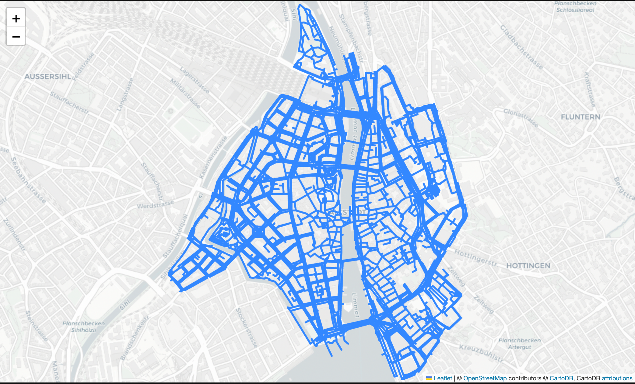
Figure 1: Graph of the area under examination (Image by Author).
We are now ready to dig into the different ways we can retrieve our data. First of all, we can get the polygon of the area we are representing as a base for our exploration. Once retrieved the data, it is then represented in a Geo Pandas data frame containing all the information of interest about the area (Figure 2). Geo Pandas is an open-source library specifically designed to extend Pandas capabilities to handle geospatial data.
In order to create any visual representation, the geometry column is used as a point of reference, in each row of this column are in fact represented all the coordinates necessary to create an object on a map (e.g. Polygon, Line, Point, MultiPolygon). In this example, Well-known text (WKT) is used as the text markup language for representing our vector geometry objects but other formats can generally be used such as GeoJSON. Additionally, each of these values in the GeoSeries is stored in a Shapely Object so that to make it as easy as possible to perform operations and transformations on it.
area = ox.geocode_to_gdf(place_name)
area.head()
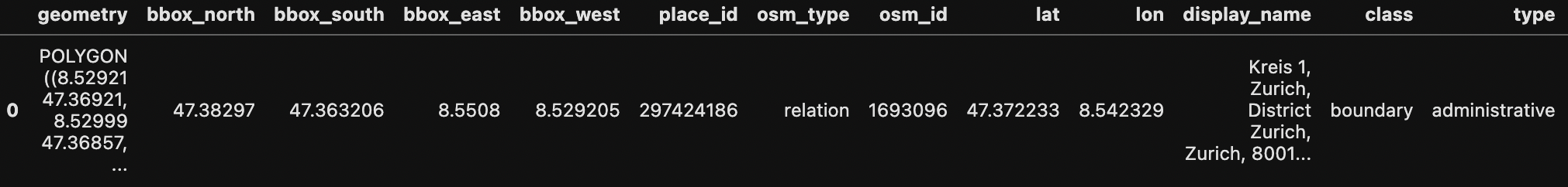
Figure 2: GeoPandas dataset example (Image by Author).
At this point, we can just repeat the same procedure to retrieve different points of interest we want to plot on our map. In this case, let’s imagine we are in Altstadt, Zurich for a holiday and we want to examine all the options we have to go to a restaurant. In order to make our research easier we can then get all the nodes and edges that represent the streets in the districts and all the buildings and restaurants available so that we can orient ourselves on the map.
buildings = ox.geometries_from_place(place_name, tags={'building':True})
restaurants = ox.geometries_from_place(place_name,
                                        tags={"amenity": "restaurant"})
nodes, edges = ox.graph_to_gdfs(graph)
Once we’ve loaded all the data, we can then plot each of the characteristics independently (Figure 3).
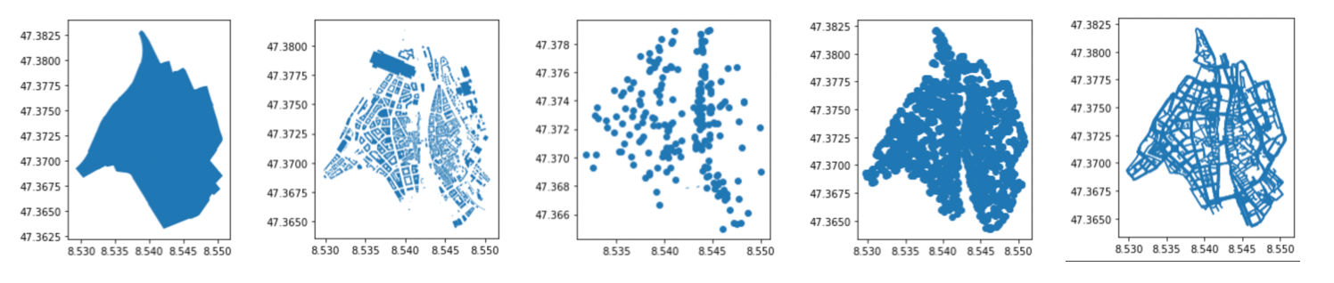
Figure 3: Area, Buildings, Restaurants, Nodes, and Edges representation (Image by Author).
Using the code below, this can finally be nicely summarized in the single graph shown below (Figure 4).
fig, ax = plt.subplots(figsize=(10, 14))
area.plot(ax=ax, facecolor='white')
edges.plot(ax=ax, linewidth=1, edgecolor='blue')
buildings.plot(ax=ax, facecolor='yellow', alpha=0.7)
restaurants.plot(ax=ax, color='red', alpha=0.9, markersize=12)
plt.tight_layout()
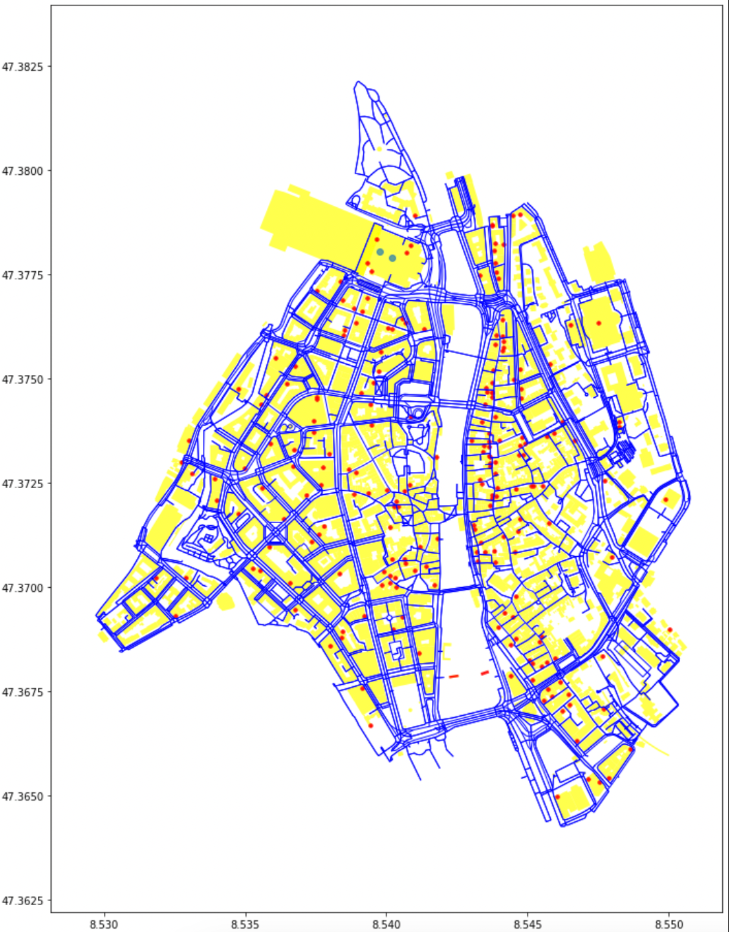
Figure 4: Analysis Summary (Image by Author).
In order to make our analysis more interactive, we could then also make use of additional libraries such as KeplerGL. KeplerGL is an open-source Geospatial toolbox developed by Uber to create high-performance web-based geo applications.
Using KeplerGL it can then be really easy for us to overlap our map on a real worldwide map and apply various transformations and filtering on it on the fly (Figure 5).
K_map = KeplerGl()
K_map.add_data(data=restaurants, name='Restaurants')
K_map.add_data(data=buildings, name='Buildings')
K_map.add_data(data=edges, name='Edges')
K_map.add_data(data=area, name='Area')
K_map.save_to_html()
Figure 5: Interactive Analysis Summary with KaplerGL (Image by Author).
Now that we have constructed our map and we have an interactive tool to examine that data we can finally try to narrow down our research to a single restaurant. In this case, we first restrict our focus to just Italian restaurants and then select Antica Roma as our place of choice.
Now, we just need to specify our initial position coordinates and place of destination to start looking for the best path to walk through (Figure 6).
it_resturants = restaurants.loc[restaurants.cuisine.str.contains('italian')
                                    .fillna(False)].dropna(axis=1, how='all')
resturant_choice = it_resturants[it_resturants['name'] == 'Antica Roma']
orig = list(graph)[993]
dest = ox.nearest_nodes(graph,
            resturant_choice['geometry'][0].xy[0][0],
            resturant_choice['geometry'][0].xy[1][0])
nodes[nodes.index == orig]
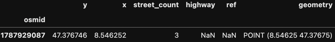
Figure 6: Starting Position representation (Image by Author).
In order to perform this task, we can make use of Networkx shortest_path function to automatically run the Dijkstra algorithm and try to optimize our path to minimize its overall length (Figure 7).
route = nx.shortest_path(graph, orig, dest, weight='length')
ox.plot_route_folium(graph, route, route_linewidth=6, node_size=0)
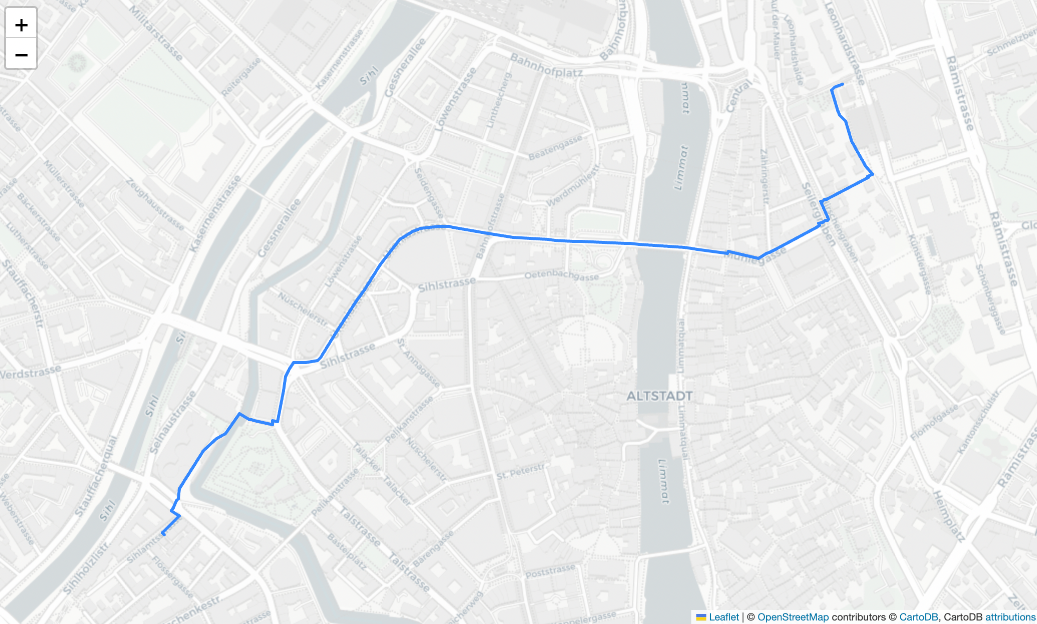
Figure 7: Shortest Path to destination (Image by Author).
Finally, to validate our research we can try to perform the same query on Google Maps and as shown below the results are pretty close to each other! (Figure 8).
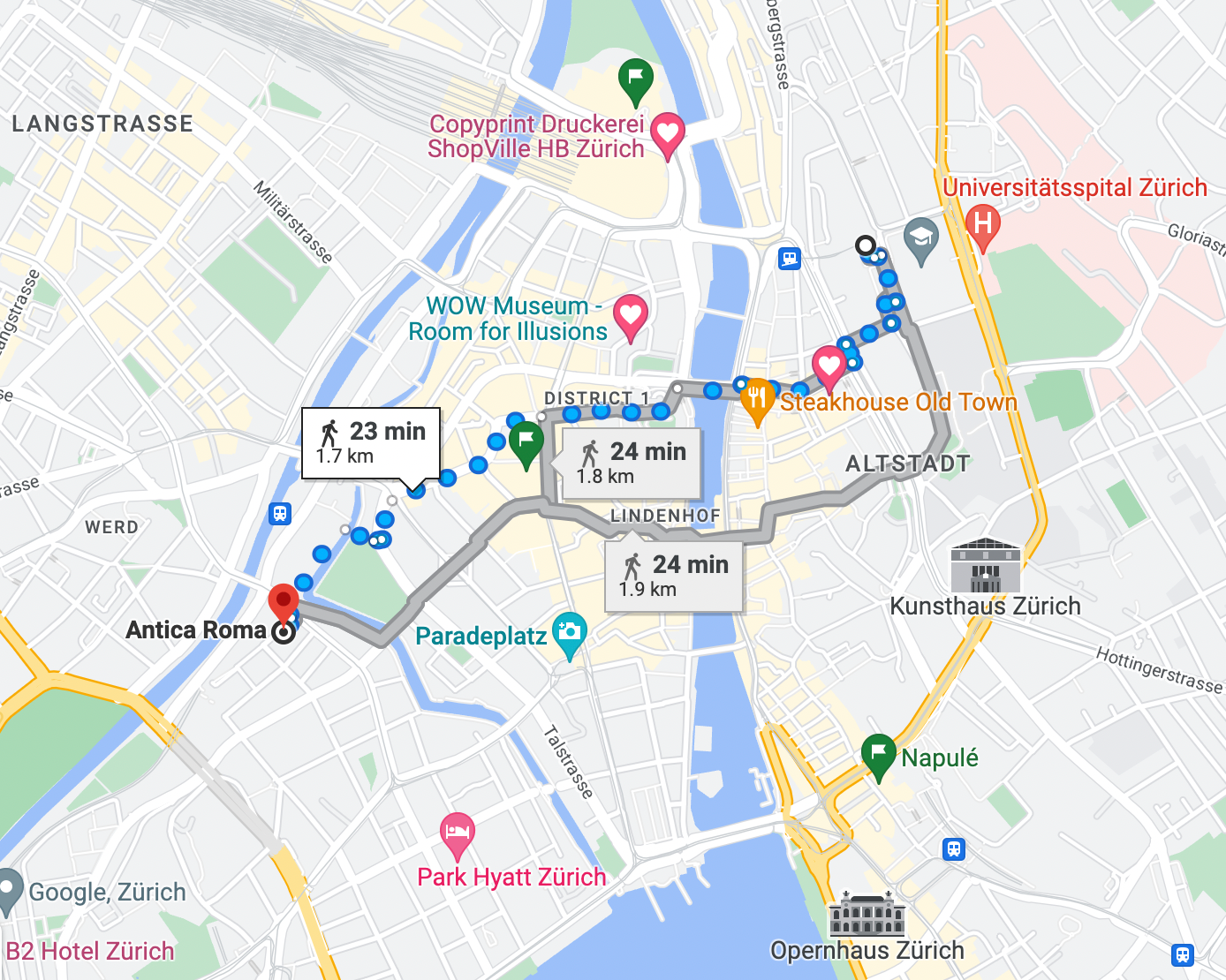
Figure 8: Google Maps Shortest Path to destination (Image by Author).
Conclusion
To summarize, in this article, we first introduced how Geospatial data is used across businesses, how it is typically stored/processed, and went through a practical example in order to identify the shortest paths between two different points. Of course, we can perform a similar kind of analysis using UI based tools such as the OpenStreetMap App or Google Maps, although learning these foundations can still be extremely valuable as they can be applied in many other forms of network-based problems (e.g. Travel Salesman Problem).
Contacts
If you want to keep updated with my latest articles and projects follow me on Medium and subscribe to my mailing list. These are some of my contacts details:
