Introduction to NannyML Model Evaluation without labels

Introduction to NannyML: Model Evaluation without labels
- Finding a way to monitor ML models performance in production when labels are not available and avoid silent failure
Introduction
ML Models Monitoring/Evaluation
Demonstration
Bibliography

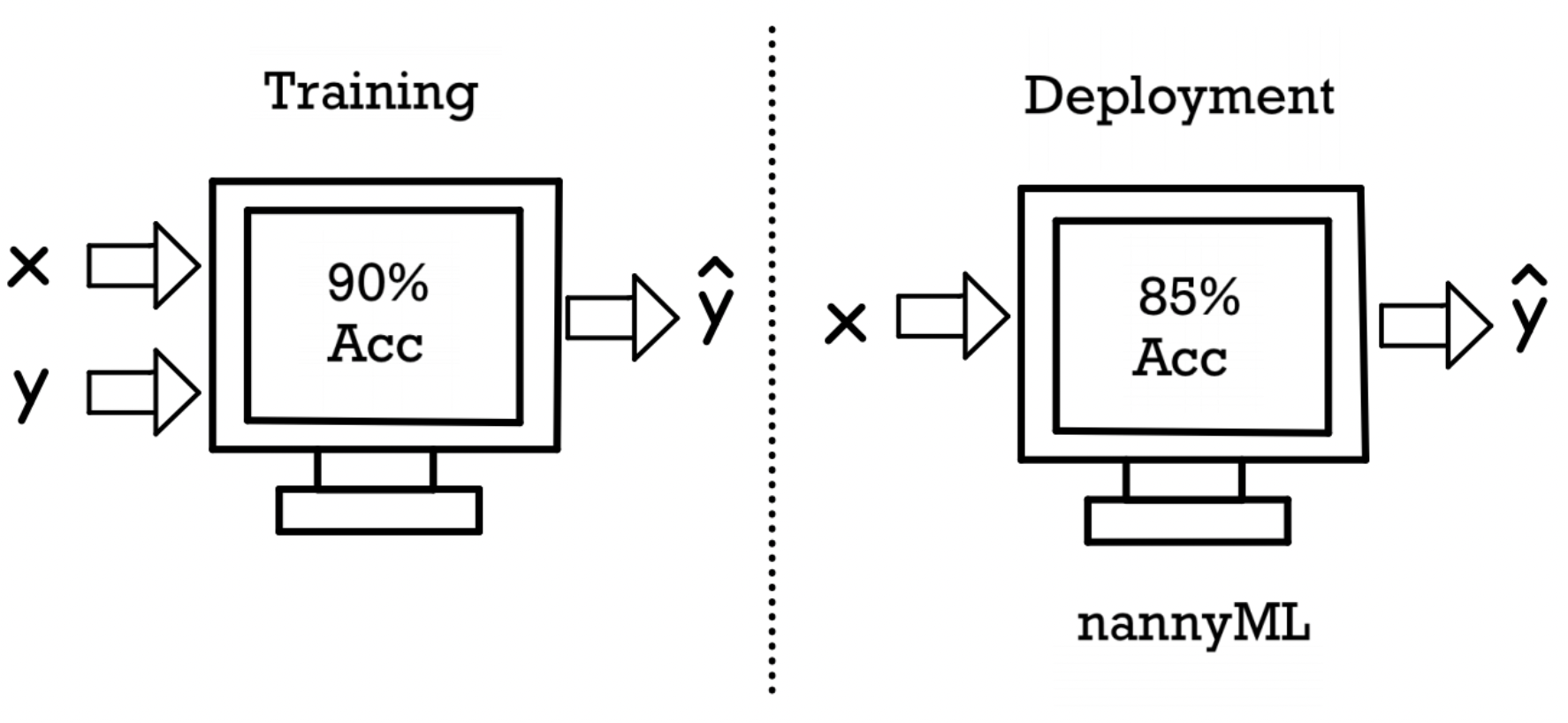
Evaluating ML Models in production without labels (Image by Author).

Introduction to NannyML: Model Evaluation without labels

Finding a way to monitor ML models performance in production when labels are not available and avoid silent failure

Introduction

Developing Machine Learning models is nowadays becoming easier and easier thanks to the different tools created by cloud providers (e.g. Amazon Sagemaker, Azure ML) and data platforms (e.g. Dataiku, DataRobot, DataBricks, etc…). Although, correctly monitoring and evaluating ML models once deployed still remains a big problem for some applications in which it can be costly (or impossible!) to gather new labels within a reasonable timeframe.

In order to try to solve this issue, NannyML was created. NannyML is an open-source Python library designed in order to make it easy to monitor drift in the distributions of our model input variables and estimate our model performance (even without labels!) thanks to the Confidence-Based Performance Estimation algorithm they developed. But first of all, why do models need to be monitored and why their performance might vary over time?

ML Models Monitoring/Evaluation

Unlike traditional software projects, which are rule-based and deterministic, ML projects are inherently probabilistic and therefore require some level of maintenance (monitoring) in the same way code quality is ensured in software development through testing.

Model Monitoring and Evaluation are an area of research falling into the MLOps subspace (Figure 1). MLOps (Machine Learning -> Operations) is a set of processes designed to transform experimental Machine Learning models into productionized services ready to make decisions in the real world. Additional information about MLOps and some of its key design patterns is available in my previous article.

Figure 1: Hidden Technical Debt in Machine Learning Systems [1]. Reposted with permission.

Some of the key reasons why we need to have a system in place to monitor and frequently re-evaluate ML models are changes in:

Data Drift: can take place when the distribution of the input features is different from the one in production (Figure 2). This change could take place suddenly due to changes in the real world or incrementally over time. Due to the nature of this shift, Data Drift does not necessarily always lead to a decrease in the performance of our model and if detected in its early stages could be taken as an opportunity to improve our model pipeline to make it more robust to these form of changes (e.g. re-training to find a better decision boundary, handle differently missing values, changes in schema, etc…).

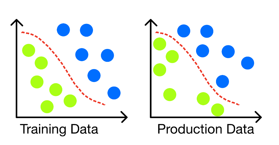
Figure 2: Data Drift without model degradation (Image by Author).

Target Drift: In the case of Target Drift, our label variable might suffer a change in its distribution and addition/removal of some of its classification categories (Figure 3).

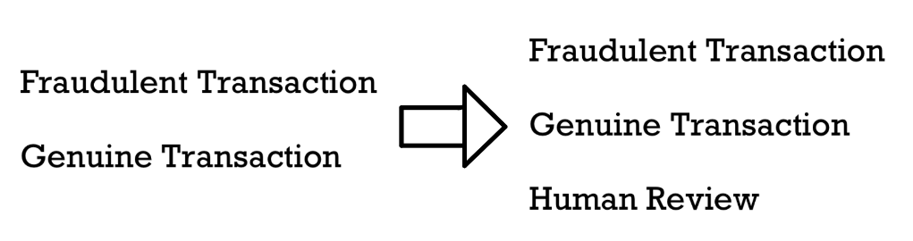
Figure 3: New categories added to our label (Image by Author).

Concept Drift: This type of drift can take place when the underlying relationship between features and labels changes (Figure 4). Making therefore the patterns learned by our model during training time no longer valid (causing an overall degradation in performance).

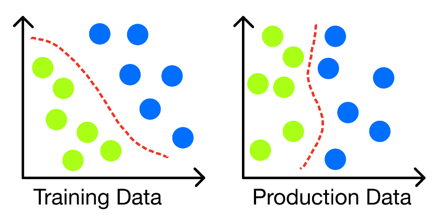
Figure 4: Concept Drift altering model decision boundary (Image by Author).

In order to try to measure drift, it is first necessary to identify a windowing approach (e.g. fixed or sliding) to select the points used for the comparison and then choose a metric to quantify the drift.

For univariate analysis, the Kolmogorov-Smirnov (KS) test can be used when working with continuous variables and the Pearson’s Chi-squared test for categorical data. In the case of multivariate analysis, we can instead first use a dimensionality reduction techniques (e.g. Principal Component Analysis, Autoencoders, etc…) to work in a lower dimensionality space and then apply a two-sample test (e.g. KS Test with Bonferroni Correction).

Once having in place a system able to identify drift it can then be important to evaluate how this can impact our model performance. In some circumstances, actual labels could be made available relatively soon and we should be able to assess performance in the same way we did for training a model, but in most cases, labels might be available just months or years after a prediction has been made (e.g. long term insurance contracts). In these circumstances, approximate signals could be fabricated as a proxy to evaluate our model, or performance estimation algorithms such as the Confidence-Based Performance Estimation algorithm developed by NannyML could be used.

Demonstration

In this article, I will walk you through a practical example in order to get started using NannyML. All the code used throughout this demonstration (and more!) is available on my GitHub and Kaggle accounts. For this example, we are going to use the Kaggle Home Equity (HMEQ) dataset [2] in order to predict if a customer is going to default or not on their loan.

First of all, we need to make sure to install NannyML.

!pip install nannyml

We are now ready to import all the necessary dependencies and visualize our dataset (Figure 5). If you are interested in learning more about what each column means, you can find additional information here.

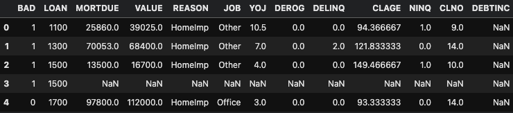
Figure 5: HMEQ Dataset (Image by Author).

Before proceeding with our analysis we need first to make sure that all categorical variables are converted into a numeric format (e.g. using One Hot Encoding), any missing value is removed, and the distribution between the two classes is as close as possible (e.g. using Oversampling and Undersampling). Once ensured that, we are then ready to split the dataset into training, test, and production sets and train a Random Forest Classifier.

At this point, we just need to check the performance of the trained model and prepare the dataset to be used by NannyML.

Considering predicting loan defaults is a quite class imbalanced problem in nature, the recall has been chosen as our metric of choice (rather than for example accuracy).

In order to prepare the dataset to be used with NannyML, the following columns have been added:

Partition: to divide the dataset into reference and analysis periods.
BAD: our target column indicating if someone has defaulted or not their loan.
Time: to make our dataset time-dependent and monitor the model performance against this dimension.
Identifier: a unique identifier for each row.
Y_Pred_Proba: a column with the prediction probabilities made by our model of if someone is going to default on their loan or not.
Y_Pred: a column with the binary predictions made by the model with a custom threshold of 75% probability.

Finally, some custom noise is added to the YOJ, MORTDUE, and CLAGE variables in order to add some arbitrary drift to the variables.

reference 0.984390243902439
analysis 0.26848249027237353

We are now finally ready to start using NannyML capabilities. First of all, a metadata variable is created to specify what kind of ML problem we are trying to solve and the columns to exclude and prioritize. Then, as shown in Figure 6, the Confidence-Based Performance Estimation (CBPE) algorithm is trained and used to make performance estimations on the analysis partition.

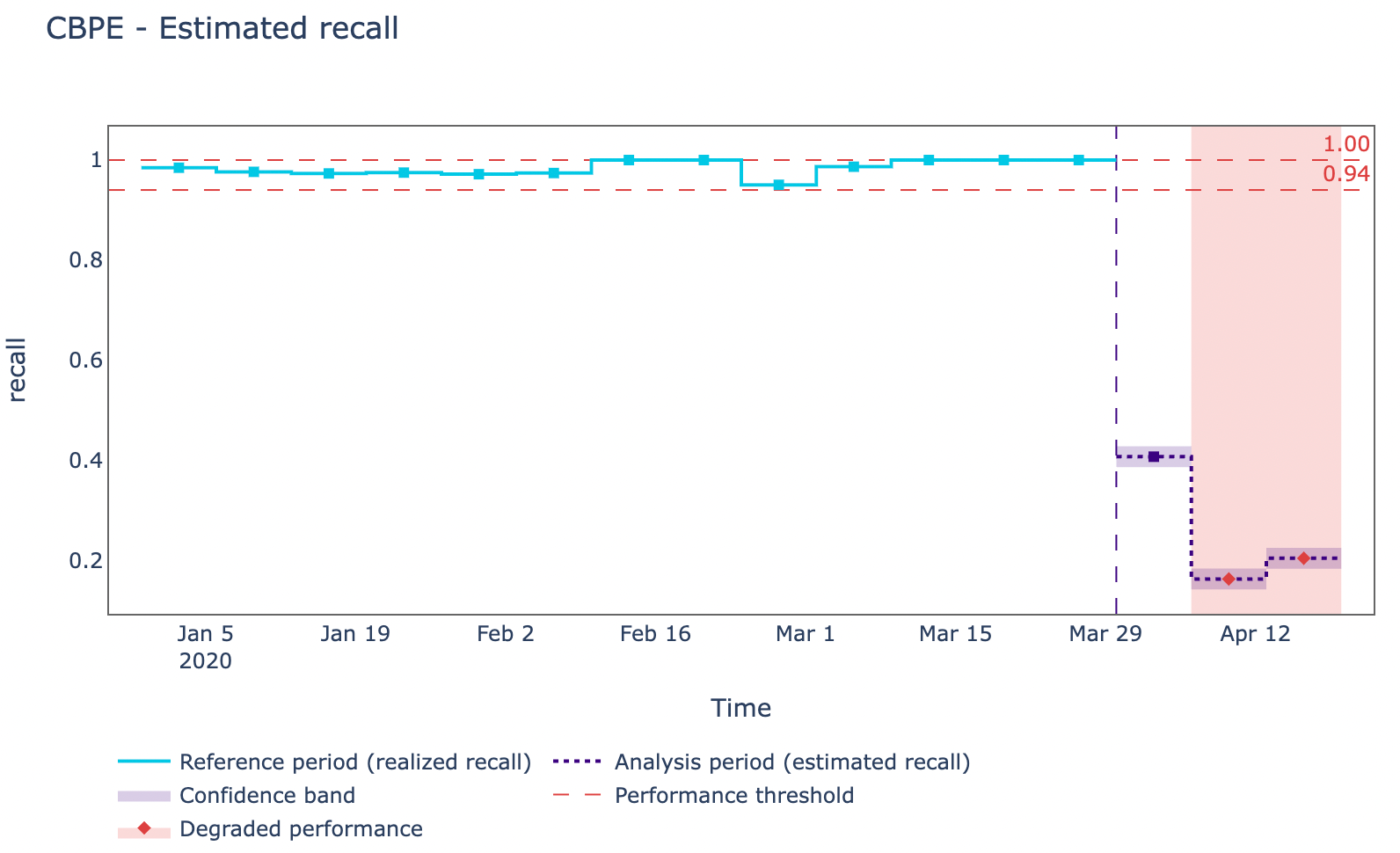
Figure 6: Confidence-Based Performance Estimation Algorithm in action (Image by Author).

Considering that in this specific case, we have the labels available we can then try to compare what recall the CBPE algorithm predicted against the actual recall of the model. As we can see from Figure 7, in this case, the algorithm was able to a good extent to foresee our model degradation throughout time.

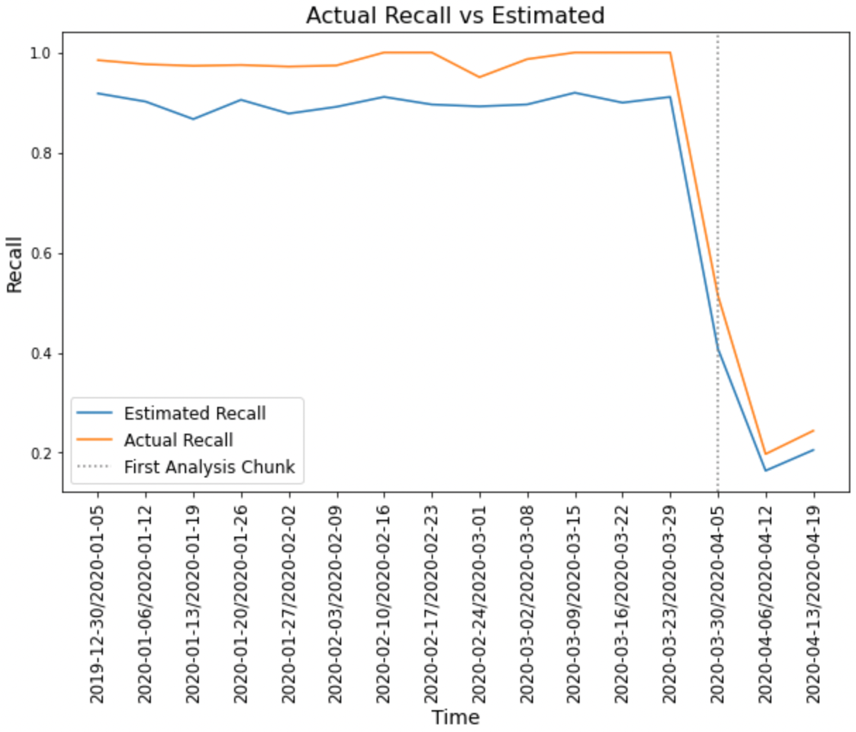
Figure 7: Actual Recall vs Estimated (Image by Author).

Now that we have validated our model is degrading over time, we can then try to take a step back and see what features might be causing this problem and are generating alerts in our monitoring system. As shown in Figure 8, YOJ, CLAGE, and MORTDUE seem to be the main causes.

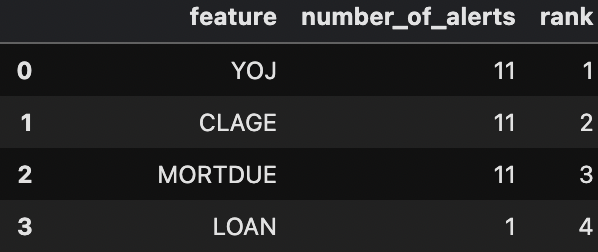
Figure 8: Number of alerts estimation (Image by Author).

Taking MORTDUE (the amount due on an existing customer mortgage) as an example, we can then go on and plot how the distribution of this feature varied against time.

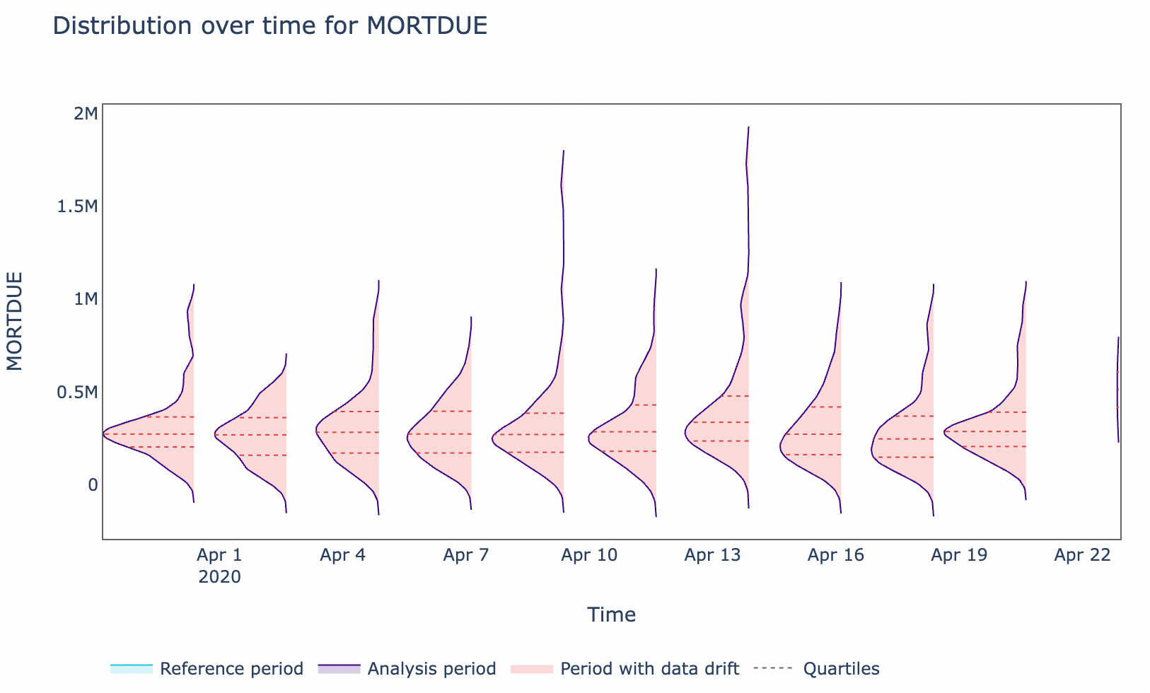
Figure 9: MORTDUE Feature distribution over time (Image by Author).

Finally, taking this analysis a step further we could then look at how the reconstruction error varied against time in the case of multivariate drift (Figure 10).

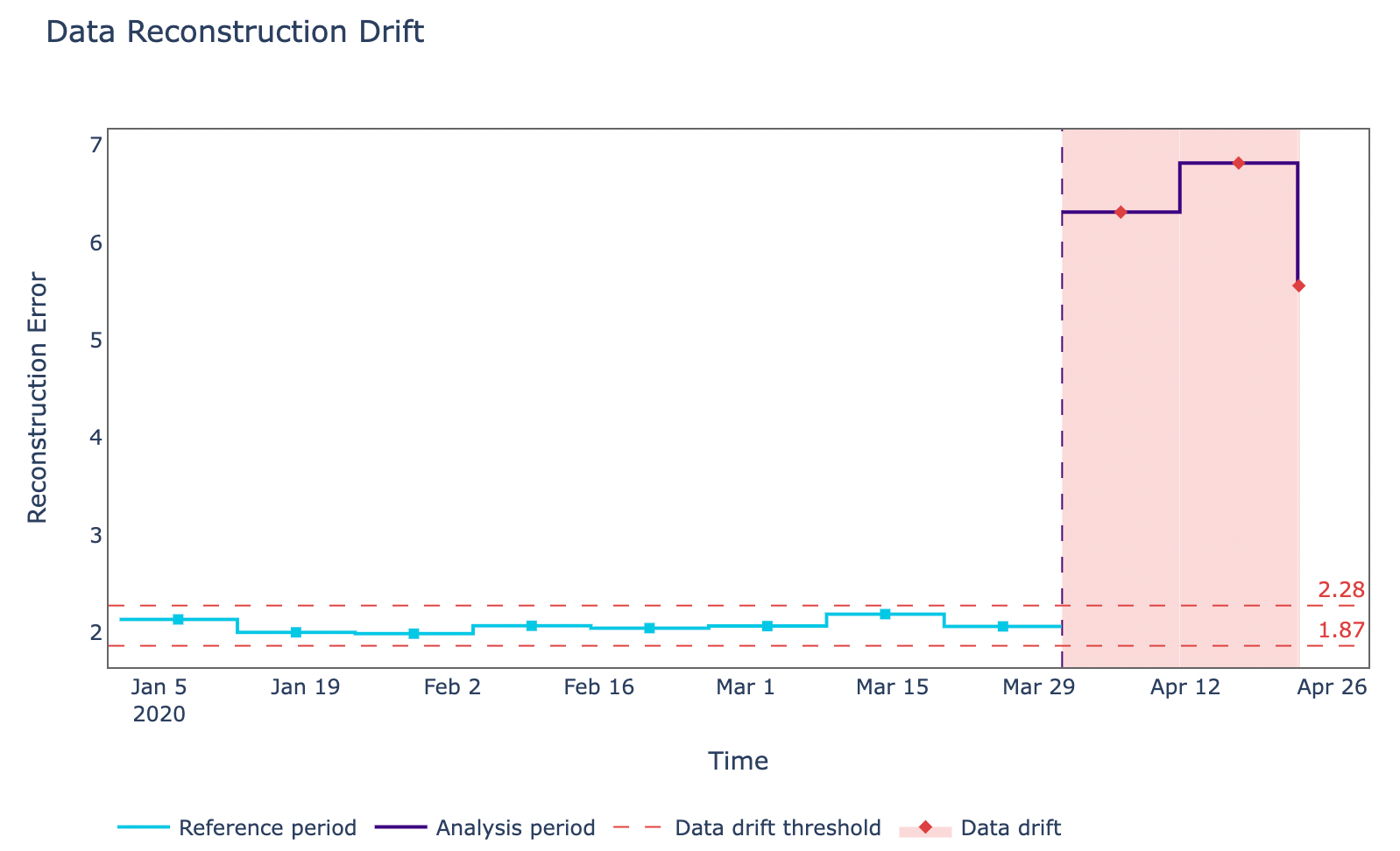
Figure 10: Multivariate Drift visualization (Image by Author).

Bibliography

[1] Hidden Technical Debt in Machine Learning Systems, D. Sculley et. al. Part of Advances in Neural Information Processing Systems 28 (NIPS 2015). Accessed at: https://papers.nips.cc/paper/2015/hash/86df7dcfd896fcaf2674f757a2463eba-Abstract.html

[2] HMEQ_Data, Predict clients who default on their loan. CC0: Public Domain. Accessed at: https://www.kaggle.com/datasets/ajay1735/hmeq-data

Contacts

If you want to keep updated with my latest articles and projects follow me on Medium and subscribe to my mailing list. These are some of my contacts details: