Contents
 (Source =https://towardsdatascience.com/support-vector-machine-vs-logistic-regression-94cc2975433f)
SVM: Feature Selection and Kernels
A Support Vector Machine (SVM) is a supervised machine learning algorithm that can be employed for both classification and regression purposes. - Noel Bambrick.
Introduction
Support Vector Machines (SVM) is a Machine Learning Algorithm which can be used for many different tasks (Figure 1). In this article, I will explain the mathematical basis to demonstrate how this algorithm works for binary classification purposes.
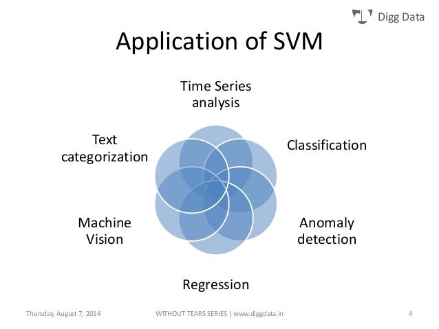
Figure 1: SVM Applications [1]
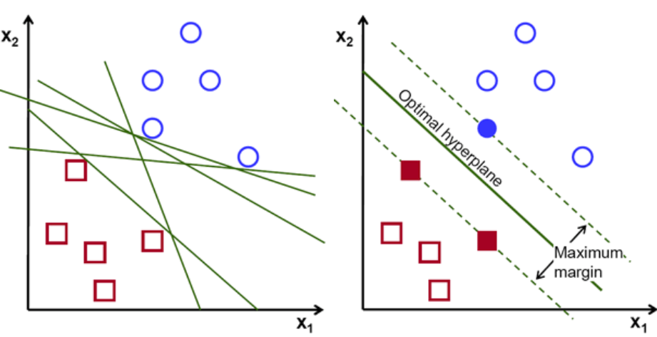
The main objective in SVM is to find the optimal hyperplane to correctly classify between data points of different classes (Figure 2). The hyperplane dimensionality is equal to the number of input features minus one (eg. when working with three feature the hyperplane will be a two-dimensional plane).
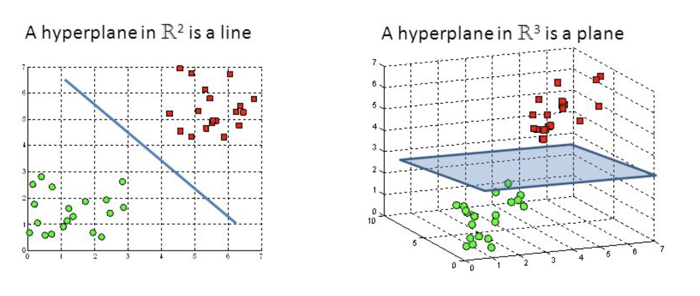
Figure 2: SVM Hyperplane [2]
Data points on one side of the hyperplane will be classified to a certain class while data points on the other side of the hyperplane will be classified to a different class (eg. green and red as in Figure 2). The distance between the hyperplane and the first point (for all the different classes) on either side of the hyperplane is a measure of sure the algorithm is about its classification decision. The bigger the distance and the more confident we can be SVM is making the right decision.
The data points closest to the hyperplane are called Support Vectors. Support Vectors determines the orientation and position of the hyperplane, in order to maximise the classifier margin (and therefore the classification score). The number of Support Vectors the SVM algorithm should use can be arbitrarily chosen depending on the applications.
Basic SVM classification can be easily implemented using the Scikit-Learn Python library in a few lines of code.
from sklearn import svm
trainedsvm = svm.SVC().fit(X_Train, Y_Train)
predictionsvm = trainedsvm.predict(X_Test)
print(confusion_matrix(Y_Test,predictionsvm))
print(classification_report(Y_Test,predictionsvm))
The are two main types of classification SVM algorithms Hard Margin and Soft Margin:
- Hard Margin: aims to find the best hyperplane without tolerating any form of misclassification.
- Soft Margin: we add a degree of tolerance in SVM. In this way we allow the model to voluntary misclassify a few data points if that can lead to identifying a hyperplane able to generalise better to unseen data.
Soft Margin SVM can be implemented in Scikit-Learn by adding a C penalty term in svm.SVC. The bigger C and the more penalty the algorithm gets when making a misclassification.
Kernel Trick
If the data we are working with is not linearly separable (therefore leading to poor linear SVM classification results), it is possible to apply a technique known as the Kernel Trick. This method is able to map our non-linear separable data into a higher dimensional space, making our data linearly separable. Using this new dimensional space SVM can then be easily implemented (Figure 3).
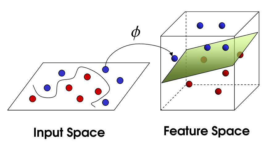
Figure 3: Kernel Trick [3]
There are many different types of Kernels which can be used to create this higher dimensional space, some examples are linear, polynomial, Sigmoid and Radial Basis Function (RBF). In Scikit-Learn a Kernel function can be specified by adding a kernel parameter in svm.SVC. An additional parameter called gamma can be included to specify the influence of the kernel on the model.
It is usually suggested to use linear kernels if the number of features is larger than the number of observations in the dataset (otherwise RBF might be a better choice).
When working with a large amount of data using RBF, speed might become a constraint to take into account.
Feature Selection
Once having fitted our linear SVM it is possible to access the classifier coefficients using .coef_ on the trained model. These weights figure the orthogonal vector coordinates orthogonal to the hyperplane. Their direction represents instead the predicted class.
Feature importance can, therefore, be determined by comparing the size of these coefficients to each other. By looking at the SVM coefficients it is, therefore, possible to identify the main features used in classification and get rid of the not important ones (which hold less variance).
Reducing the number of features in Machine Learning plays a really important role especially when working with large datasets. This can in fact: speed up training, avoid overfitting and ultimately lead to better classification results thanks to the reduced noise in the data.
In Figure 4 are shown the main features I identified using SVM on the Pima Indians Diabetes Database. In green are shown all the features corresponding to the negative coefficients and in blue the positive ones. If you want to find out more about it, all my code is freely available on my Kaggle and GitHub profiles.
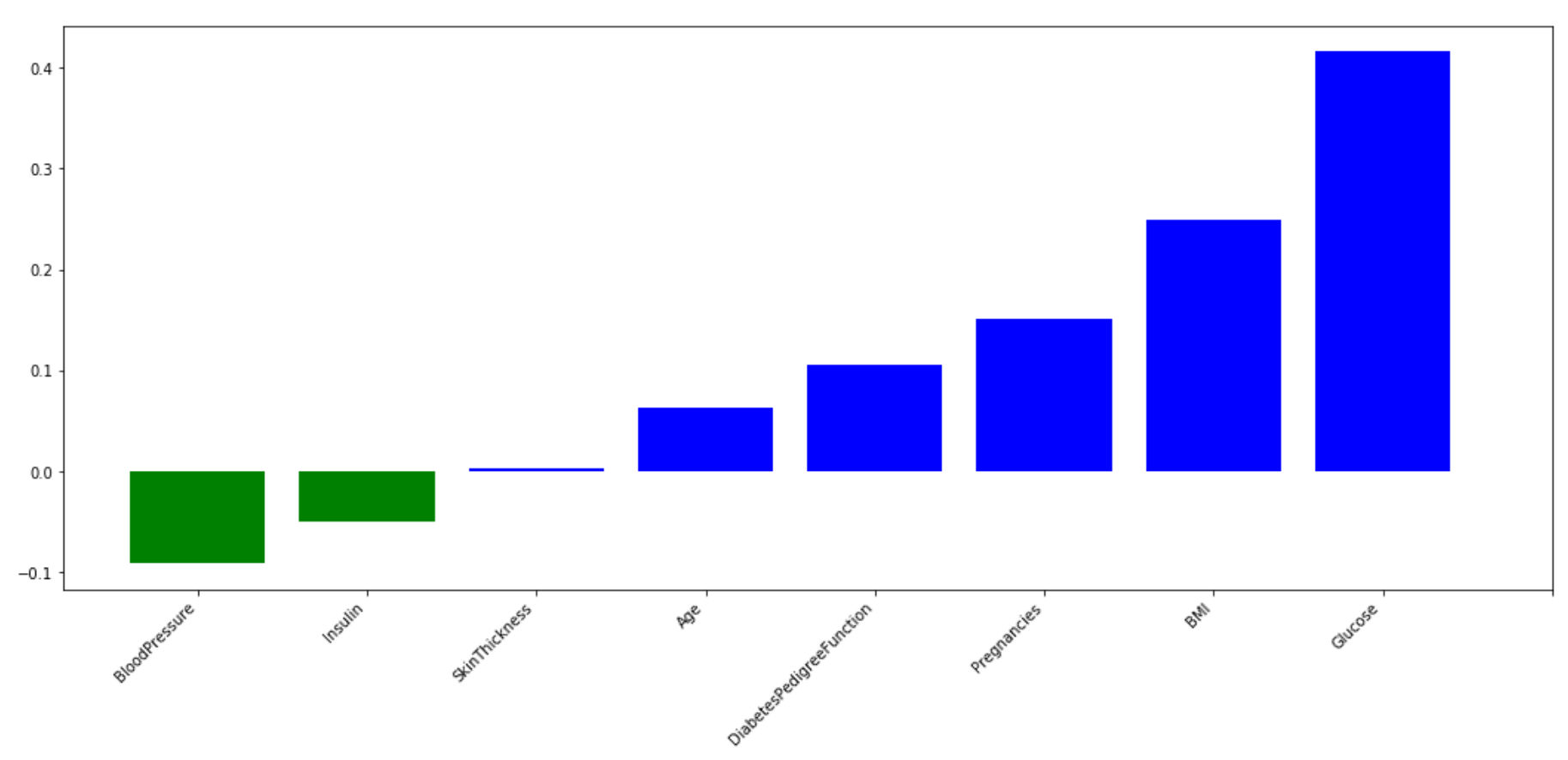
Figure 4: Feature Importance using SVM
Mathematics
If you would like to dig into the Mathematics behind SVM, I have left here a lecture from Patrick Winston available on the MIT OpenCourseWare YouTube channel [4]. This lecture illustrates how to derive the SVM decision rules and which mathematical constraints are to apply using Lagrangian Multipliers.
Video 1: MIT OpenCourseWare [4]
Bibliography
[1] Support Vector Machine without tears, Ankit Sharma. Accessed at: https://www.slideshare.net/ankitksharma/svm-37753690
[2] Support Vector Machine — Introduction to Machine Learning Algorithms, Rohith Gandhi. Accessed at: https://towardsdatascience.com/support-vector-machine-introduction-to-machine-learning-algorithms-934a444fca47
[3] Support vector machines, Jeremy Jordan. Accessed at: https://www.jeremyjordan.me/support-vector-machines/
[4] MIT OpenCourseWare, 16. Learning: Support Vector Machines. Accessed at: https://www.youtube.com/watch?v=_PwhiWxHK8o
Contacts
If you want to keep updated with my latest articles and projects follow me on Medium and subscribe to my mailing list. These are some of my contacts details:
